How To Remove Minus Sign In Excel Pivot
To hide all of the expandcollapse buttons in the pivot table. Please enter this formula.
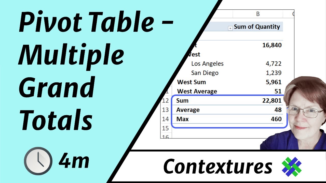
Multiple Grand Totals In Excel Pivot Table Youtube
Then select cell F1 and drag the fill handle across to the range cells which.
How to remove minus sign in excel pivot. Select the dataset from which you want to remove the dashes Hold the Control key and then press the H key. The formula will be. You can do a custom format cells that will display the opposite sign.
Now this was not the end of the world but I really only wanted positive numbers to show in my Pivot Table. In the other scenario when your data is completely numeric and you want to have a minus sign before each value just multiply them with -1 as show below. In the Format Cells dialog under Number tab select Number from the Category list and the go to the right section.
For removing the plus or minus sign please select the rows or columns which you have added plus or minus sign. 2 Above formulas only can work when there are only numeric characters and plus or minus sign. Click the Display tab In the Display section remove the check mark from Show ExpandCollapse Buttons.
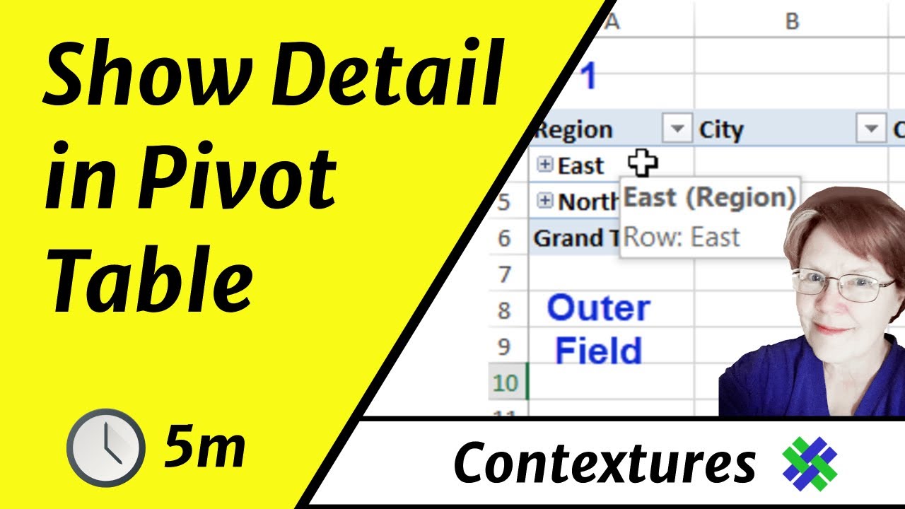
Hide expand and collapse buttons with PivotTable Options. Remove the check mark from the option Show. In the PivotTable Options dialog under the Display tab uncheck Show expandcollapse buttons in the Display section see.
Raw data for excel practice download. Enter the formula below we will just concatenate a minus sign at the beginning of the value as show below. Select the numbers and then right click to shown the context menu and select Format Cells.
And click the Plus sign the hidden rows or columns are showing at once. This change will hide the ExpandCollapse buttons to the left of the outer Row Labels and Column Labels. We now have the number without the negative sign.
Select the cells involved right-click Format Cells Number tab click Custom and then in the small box just under the word Type on the right side enter this. Putting this together with the LEFT function and adding minus 1 to the formula pulls only 5 of the first 6 characters of the cell leaving the negative sign behind. Right click a cell in the pivot table and choose PivotTable Options from the context menu see screenshot.
In the Find what field type the dash symbol -. I hope you understood how to remove unwanted characters from the text using SUBSTITUTE function in Excel. Right-click any cell in the pivot table.
This will open the Find and Replace dialog box. Hide Excel Pivot Table Buttons. Right-click a cell in the pivot table and in the pop up menu click PivotTable Options.
In the pop-up menu click PivotTable Options. To remove the negative sign from the numbers here is a simple ABS function please do as follows. 1 If your data includes minus sign you can use this formula SUBSTITUTE A1-0 to remove the minus sign of each cells.
Remove plus sign or minus sign of each cell with Kutools for Excel. ABS A1 into a blank cell and press Enter key and the negative sign has been removed. In the PivotTable Options dialog box click the Display tab.
As you can see the value is cleaned in both the cases whether it is single space or any other character. I was creating a Pivot Table this week one of many and it contained negative numbers. Click the minus sign the selected rows or column are hidden immediately.
Inserting -1 into the formula multiplies the number by negative 1 therefore placing the negative sign in front of it. LEFTA5 grabs the single space code in the formula using LEFT CODE function and giving as input to char function to replace it with an empty string. I did not want the either of the zeros or the negative numbers to be visible.
Hello Excellers I have a handy Excel Pivot Table Tip for you today. Remove leading minus sign from cell with Format Cells 1.

Pivot Table Pivot Table Year Over Year By Month Exceljet

How To Hide Expand Collapse Buttons In Pivot Table
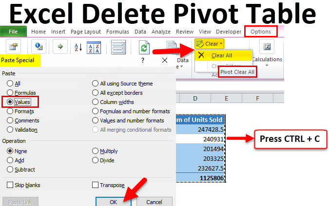
How To Delete A Pivot Table Methods Step By Step Tutorials
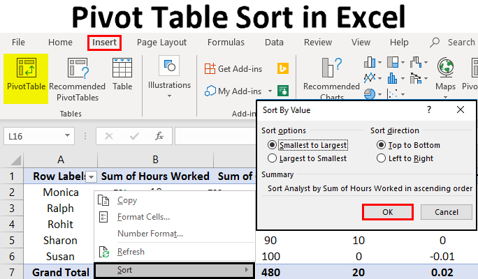
Pivot Table Sort In Excel How To Sort Pivot Table Columns And Rows
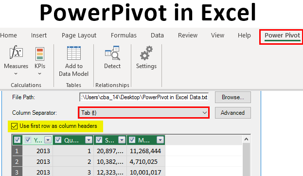
Powerpivot In Excel Examples On How To Activate Powerpivot In Excel
Excel Pivot Tables Quick Guide Tutorialspoint
![]()
Icon Sets In A Pivot Table Myexcelonline

Pivot Table To Create List Of Unique Items Remove Duplicates Excel Computer Help Pivot Table

Excel Formulas Simple Formulas Excel Formula Subtraction Microsoft Excel
Expand And Collapse Details In An Excel Pivot Table Youtube
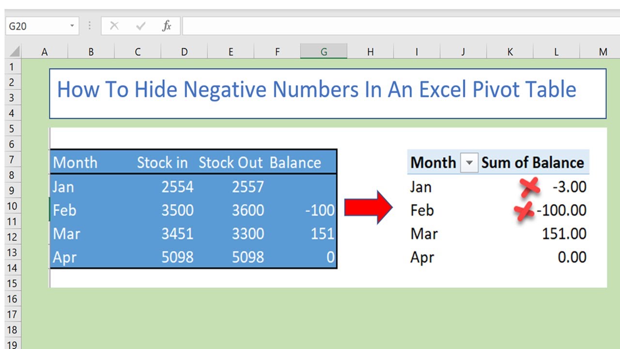
Hide Negative Numbers In Excel Pivot Table Youtube
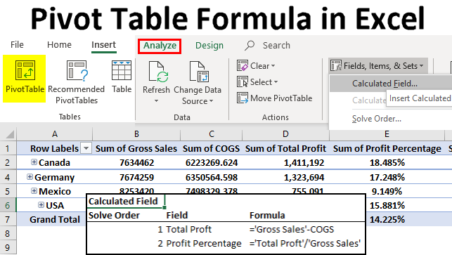
Pivot Table Formula In Excel Steps To Use Pivot Table Formula In Excel
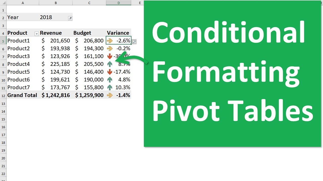
How To Apply Conditional Formatting To Pivot Tables Youtube
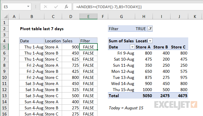
Pivot Table Pivot Table Last 7 Days Exceljet

Pivot Table Dialog Box Pivot Table Excel Excel Formula

Pivot Table Excel The 2020 Tutorial Earn Excel
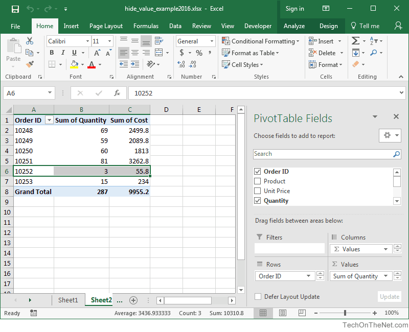
Ms Excel 2016 How To Hide A Value In A Pivot Table

Pivot Tables In Excel How To Create Use The Excel Pivottable Function
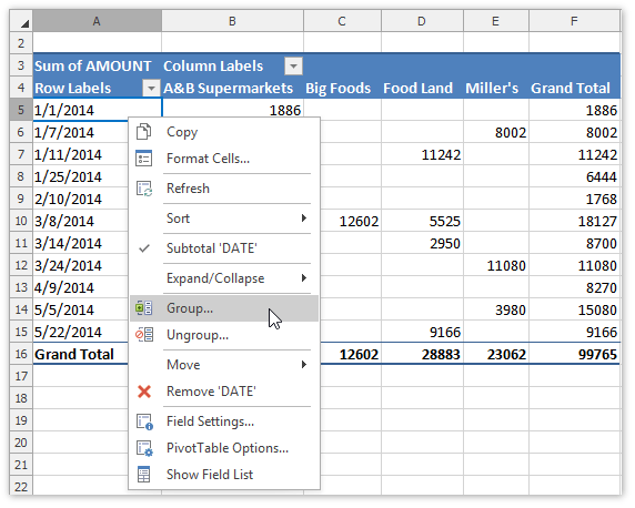
Group Items In A Pivot Table Devexpress End User Documentation